Refactoring legacy SQL to dbt
Introduction
You may have already learned how to build dbt models from scratch. But in reality, you probably already have some queries or stored procedures that power analyses and dashboards, and now you’re wondering how to port those into dbt.
There are two parts to accomplish this: migration and refactoring. In this guide we’re going to learn a process to help us turn legacy SQL code into modular dbt models.
When migrating and refactoring code, it’s of course important to stay organized. We'll do this by following several steps:
- Migrate your code 1:1 into dbt
- Implement dbt sources rather than referencing raw database tables
- Choose a refactoring strategy
- Implement CTE groupings and cosmetic cleanup
- Separate data transformations into standardized layers
- Audit the output of dbt models vs legacy SQL
Let's get into it!
This guide is excerpted from the new dbt Learn On-demand Course, "Refactoring SQL for Modularity" - if you're curious, pick up the free refactoring course here, which includes example and practice refactoring projects. Or for a more in-depth look at migrating DDL and DML from stored procedures, refer to theMigrate from stored procedures guide.
Migrate your existing SQL code
Your goal in this initial step is simply to use dbt to run your existing SQL transformation, with as few modifications as possible. This will give you a solid base to work from.
While refactoring you'll be moving around a lot of logic, but ideally you won't be changing the logic. More changes = more auditing work, so if you come across anything you'd like to fix, try your best to card that up for another task after refactoring! We'll save the bulk of our auditing for the end when we've finalized our legacy-to-dbt model restructuring.
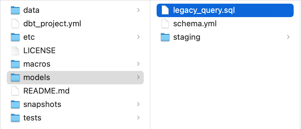
To get going, you'll copy your legacy SQL query into your dbt project, by saving it in a .sql file under the /models directory of your project.
Once you've copied it over, you'll want to dbt run to execute the query and populate the table in your warehouse.
If this is your first time running dbt, you may want to start with the Introduction to dbt and the earlier sections of the quickstart guide before diving into refactoring.
This step may sound simple, but if you're porting over an existing set of SQL transformations to a new SQL dialect, you will need to consider how your legacy SQL dialect differs from your new SQL flavor, and you may need to modify your legacy code to get it to run at all.
This will commonly happen if you're migrating from a stored procedure workflow on a legacy database into dbt + a cloud data warehouse.
Functions that you were using previously may not exist, or their syntax may shift slightly between SQL dialects.
If you're not migrating data warehouses at the moment, then you can keep your SQL syntax the same. You have access to the exact same SQL dialect inside of dbt that you have querying directly from your warehouse.
Create sources from table references
To query from your data warehouse, we recommend creating sources in dbt rather than querying the database table directly.
This allows you to call the same table in multiple places with {{ src('my_source', 'my_table') }} rather than my_database.my_schema.my_table.
We start here for several reasons:
Source freshness reporting
Using sources unlocks the ability to run source freshness reporting to make sure your raw data isn't stale.
Easy dependency tracing
If you're migrating multiple stored procedures into dbt, with sources you can see which queries depend on the same raw tables.
This allows you to consolidate modeling work on those base tables, rather than calling them separately in multiple places.
Build the habit of analytics-as-code
Sources are an easy way to get your feet wet using config files to define aspects of your transformation pipeline.
sources:
  - name: jaffle_shop
    tables:
      - name: orders
      - name: customers
With a few lines of code in a .yml file in your dbt project's /models subfolder, you can now version control how your data sources (Snowplow, Shopify, etc) map to actual database tables.
For example, let's say you migrate from one ETL tool to another, and the new tool writes to a new schema in your warehouse. dbt sources allow you to make that update in a single config file, and flip on the change with one pull request to your dbt project.
Choose a refactoring strategy
There are two ways you can choose to refactor: in-place or alongside.
In-place refactoring
Means that you will work directly on the SQL script that you ported over in the first step.
You'll move it into a /marts subfolder within your project's /models folder and go to town.
Pros:
- You won't have any old models to delete once refactoring is done.
Cons:
- More pressure to get it right the first time, especially if you've referenced this model from any BI tool or downstream process.
- Harder to audit, since you've overwritten your audit comparison model.
- Requires navigating through Git commits to see what code you've changed throughout.
Alongside refactoring
Means that you will copy your model to a /marts folder, and work on changes on that copy.
Pros:
- Less impact on end users - anything that is referencing the model you're refactoring can keep that reference until you can safely deprecate that model.
- Less pressure to get it right the first time, meaning you can push/merge smaller PRs. This is better for you and your reviewers.
- You can audit easier by running the old and new models in your dev branch and comparing the results. This ensures the datasets you're comparing have the same or very close to the same records.
- You can look at old code more easily, as it has not been changed.
- You can decide when the old model is ready to be deprecated.
Cons:
- You'll have the old file(s) in your project until you can deprecate them - running side-by-side like this can feel duplicative, and may be a headache to manage if you're migrating a number of queries in bulk.
We generally recommend the alongside approach, which we'll follow in this tutorial.
Implement CTE groupings
Once you choose your refactoring strategy, you'll want to do some cosmetic cleanups according to your data modeling best practices and start moving code into CTE groupings. This will give you a head start on porting SQL snippets from CTEs into modular dbt data models.
What's a CTE?
CTE stands for “Common Table Expression”, which is a temporary result set available for use until the end of SQL script execution. Using the with keyword at the top of a query allows us to use CTEs in our code.
Inside of the model we're refactoring, we’re going to use a 4-part layout:
- 'Import' CTEs
- 'Logical' CTEs
- A 'Final' CTE
- A simple SELECT statement
In practice this looks like:
with

import_orders as (

    -- query only non-test orders
    select * from {{ source('jaffle_shop', 'orders') }}
    where amount > 0
),

import_customers as (
    select * from {{ source('jaffle_shop', 'customers') }}
),

logical_cte_1 as (

    -- perform some math on import_orders

),

logical_cte_2 as (

    -- perform some math on import_customers
),

final_cte as (

    -- join together logical_cte_1 and logical_cte_2
)

select * from final_cte
Notice there are no nested queries here, which makes reading our logic much more straightforward. If a query needs to be nested, it's just a new CTE that references the previous CTE.
1. Import CTEs
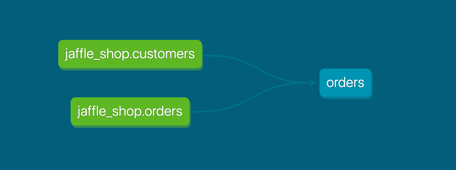
Let's start with our components, and identify raw data that is being used in our analysis. For this exercise, the components are three sources:
- jaffle_shop.customers
- jaffle_shop.orders
- stripe.payment
Let's make a CTE for each of these under the Import CTEs comment. These import CTEs should be only simple select * statements, but can have filters if necessary.
We'll cover that later - for now, just use select * from {{ source('schema', 'table') }} for each, with the appropriate reference. Then, we will switch out all hard-coded references with our import CTE names.
2. Logical CTEs
Logical CTEs contain unique transformations used to generate the final product, and we want to separate these into logical blocks. To identify our logical CTEs, we will follow subqueries in order.
If a subquery has nested subqueries, we will want to continue moving down until we get to the first layer, then pull out the subqueries in order as CTEs, making our way back to the final select statement.
Name these CTEs as the alias that the subquery was given - you can rename it later, but for now it is best to make as few changes as possible.
If the script is particularly complicated, it's worth it to go through once you're finished pulling out subqueries and follow the CTEs to make sure they happen in an order that makes sense for the end result.
3. Final CTE
The previous process usually results in a select statement that is left over at the end - this select statement can be moved into its own CTE called the final CTE, or can be named something that is inherent for others to understand. This CTE determines the final product of the model.
4. Simple SELECT statement
After you have moved everything into CTEs, you'll want to write a select * from final (or something similar, depending on your final CTE name) at the end of the model.
This allows anyone after us to easily step through the CTEs when troubleshooting, rather than having to untangle nested queries.
For more background on CTEs, check out the dbt Labs style guide.
Port CTEs to individual data models
Rather than keep our SQL code confined to one long SQL file, we'll now start splitting it into modular + reusable dbt data models.
Internally at dbt Labs, we follow roughly this data modeling technique and we structure our dbt projects accordingly.
We'll follow those structures in this walkthrough, but your team's conventions may of course differ from ours.
Identifying staging models
To identify our staging models, we want to look at the things we've imported in our import CTEs.
For us, that's customers, orders, and payments. We want to look at the transformations that can occur within each of these sources without needing to be joined to each other, and then we want to make components out of those so they can be our building blocks for further development.
CTEs or intermediate models
Our left-over logic can then be split into steps that are more easily understandable.
We'll start by using CTEs, but when a model becomes complex or can be divided out into reusable components you may consider an intermediate model.
Intermediate models are optional and are not always needed, but do help when you have large data flows coming together.
Final model
Our final model accomplishes the result set we want, and it uses the components we've built. By this point we've identified what we think should stay in our final model.
Data model auditing
We'll want to audit our results using the dbt audit_helper package.
Under the hood, it generates comparison queries between our before and after states, so that we can compare our original query results to our refactored results to identify differences.
Sure, we could write our own query manually to audit these models, but using the dbt audit_helper package gives us a head start and allows us to identify variances more quickly.
Ready for refactoring practice?
Head to the free on-demand course, Refactoring from Procedural SQL to dbt for a more in-depth refactoring example + a practice refactoring problem to test your skills.
Questions on this guide or the course? Drop a note in #learn-on-demand in dbt Community Slack.

